Posts

Week starting 07/15/19 (Week 7)

Image
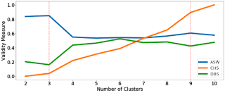
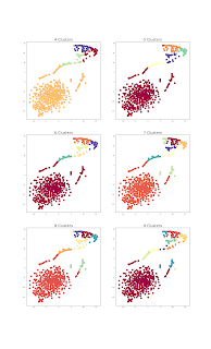
This week I started clustering the data after using multiple distance algorithms on the v, specifically Dynamic Time Warping (DTW), Fourier Coefficients, Autocorrelation, and the Euclidean Distance. After the clusters have been calculated, a cluster validity algorithm have to be run in order to determine the optimal number of clusters. The cluster validity algorithm included the Average Silhouette Width (ASW), the Calinski Harabasz Score (CHS), and the Davies-Bouldin Score (DBS). These metrics are set up in such a way that we want to obtain the highest Average Silhouette Width (ASW) and Calinski Harabasz Score (CHS) and the lowest Davies-Bouldin Score (DBS). For the variable air temperature, the best results so far have come from running DTW and running that through a dimensionality reduction algorithm called Uniform Manifold Approximation and Projection (UMAP). Result of the silhouette width where the red line is the average (Left) and visual representation of data with t

Week 6

We continued to research distance measurements and figure out how they work. We K-means to cluster the net ecosystem exchange values from 659 sights. Then I began to calculate the dynamic time warping distances from all of the sites so that I can use K-means to cluster the values to visualize the similarity of the net ecosystem values.

Week starting 07/08/19 (Week 6)

Image
This week I started to cluster the data in order to determine where there will most likely be similarities. I have used both Umap and Tsne in combination with Kmeans prediction. The next step is to use cluster validity metrics such as Associated Silhouette Width in order to determine which cluster is best for the given data. Below are the results of Tsne (top) and Umap (bottom). In addition to this, work is being done with the distance measures that were described before.

Week Starting 07/01/19 (Week 5)

I reported my findings to the Scientific Data Management group with the slides that can be found here . This presentation was a basic overview of what I have accomplished over the past few weeks. In addition to this, I wrote a paper that gave a detailed description of the project as well as some work that has been done this far and what still needs to be done which can be found here . As for the code, not much has changed, but there certainly was some minor details that were adjusted to more accurately describe what exactly is going on.

Week 5

Image
We gave presentations on our progress so far and wrote a paper about the materials and the methods that will be used for the rest of this internship. I was able to get the half-hourly data to be split into sets of 48 elements using the split function. Once I had done that, I calculated euclidean distances between each of these sets of 48 to get 365 distances which was then placed into a vector to be plotted. The comparisons so far were with AT_Neu_NEE_f 2002, 2003, 2004. The 2002 dataset was missing the first 16 days worth of data, therefore those vectors that compared with 2002 had less elements and when plotted had to be shifted as to not show any data for the first 16 days. We will continue these calculations with other variables and use other methods to compare the datasets.

Week 4 Weekend

Image
This weekend my friend from High School, Colby, came to visit.  On Saturday we walked the Trail's End. which was incredible, even if it was a lot more hiking than it we expected it to be. After that we ended up at Pride inadvertently. On Sunday we went to the Point Bonita lighthouse. The view was spectacular, but it was incredibly windy, so we were very cold the whole time. Then we ended up at a beach and stayed there for half an hour or so until the temperature yet again got the better of us. Our final destination in San Fransisco was to the Full House building (for the second time)

Week Starting 6/24/19 (Week 4)

Image
This week we started working with multiple different methods for determine similarities in the FLUXNET dataset. So far I have created graphs that compare several variables such as Net Ecosystem Exchange, Heat flux, and more for both hourly and daily values. I also worked on a presentation of my progress. Below are the graphs hourly and daily Net Ecosystem Exchange of three Italian towers in 2002. I also created graphs for the absolute value of each difference. Below are the differences between the towers with respect to the Net Ecosystem Exchange.